Clear costs: How we used data aggregation to understand our Cost of Goods Sold

Understanding COGS (cost of goods sold) is key to running any successful business. As a SaaS company, we need an understanding of not only our overall COGS but also how much each of our product features is contributing to COGS with an accurate cost allocation at the customer level. This helps our engineering squads design more cost-efficient architecture and enables our business teams to make more informed pricing decisions. 

This article explores the tools mParticle uses and the pipeline we built to gain insight into our AWS spending. It also dives into how we solved core problems to bring key datasets together, and how this helped us identify the core services that were resulting in unnecessary spend.

To understand how much our customers were costing us, we first needed to know how much we were spending in general. Major cloud providers like Azure, AWS, and GCP all provide insights into the costs incurred through the use of their services. 

mParticle uses AWS and from the AWS Cost Explorer, we were able to get a breakdown of how much we were spending by AWS service (e.g., S3, SQS, EC2 usage, etc). In order to associate these costs with our customers, however, we needed more information.

With the raw AWS data alone, there was no clear way to associate service costs with individual customers, since for example, we may have multiple customer’s data flowing through the same SQS queue with logical isolation. Another issue we faced was during compute-intensive workloads, we wanted to track CPU consumption by customer, though the raw AWS data only allowed us to see how much we were spending at the aggregate level.

Using AWS Cost & Usage Reports (CUR) we were able to access all of our cost data.

Theoretically, by joining this information to other datasets as needed, we could get the additional information we were looking for.

To accomplish this data aggregation task, we developed a custom library called CustomerAccountant which gives mParticle services a way to cleanly provide the extra cost breakdown information per customer when using these AWS services. For example, data from many customers may flow through a single SQS queue before being split off to do other things. SQS charges by total messages and message size, and thus we use our CustomerAccountant to track the number of messages and total byte size used by each customer. The CustomerAccountant regularly sends this information from the service into a Kinesis Firehose that delivers this information into our BI Redshift cluster.

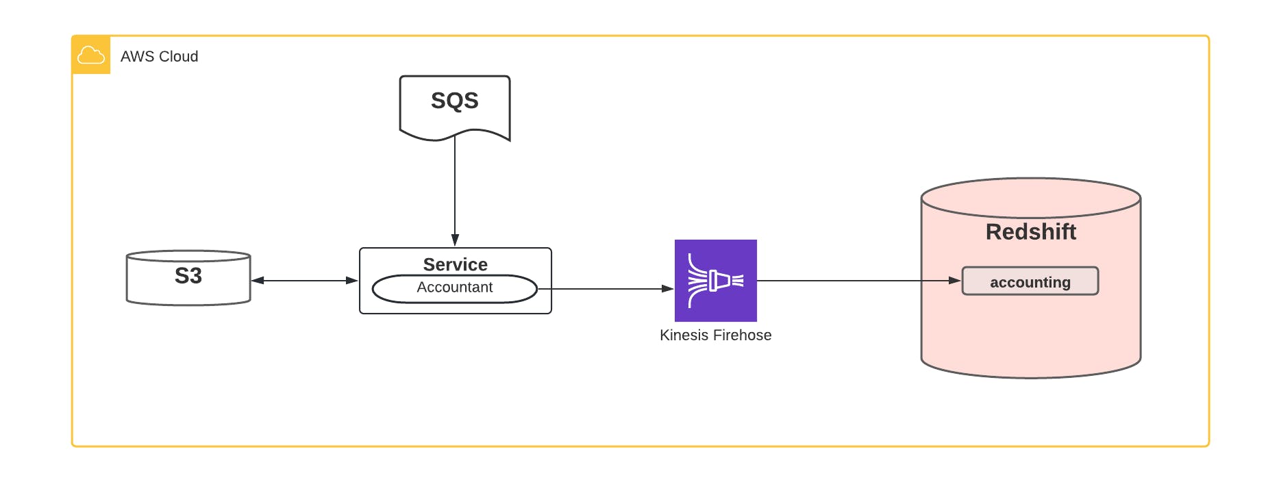
What does the CustomerAccountant information look like? There are a few important things we care about, namely: 

• Who is the customer in question?
• Which service or resource did they use?
• How much of this resource did they consume? 
• When did it take place?

So the data the CustomerAccountant might record for SQS message publishing could look like:
- CustomerID = 1234 

- Service = mParticle service A

- Resource = SQS

- Resource kind = Bytes written

- Consumption = 200.0 (bytes)

- Datetime = 2022-01-28 10:20:00

But what if we are recording CPU consumption? We still record the same set of information, but consumption isn’t necessarily tracked in bytes in this case. Here we would track consumption in milliseconds, and since this remains a numerical value, our dataset remains consistent: 

- CustomerID = 2345

- Service = mParticle service A

- Resource = CPU

- Resource kind = Time

- Consumption = 4205.0 (ms)

- Datetime = 2022-01-28 10:20:00

With the CustomerAccountant library, each of our engineering squads are responsible for instrumenting it to track necessary metrics to understand the usage of their components. We’ve made this a requirement for releasing any product into production.

Having a dataset with common fields keeps things simple both while ingesting the data into Kinesis and while consuming the data from Redshift. All of the CustomerAccountant data ends up in an accounting table in our BI Redshift cluster.

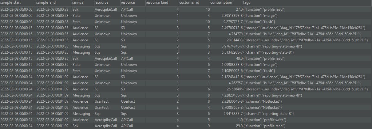
This accounting table has grown very large over time - billions of rows - due to the sheer volume of data being collected, because each container instance runs its own CustomerAccountant and sends data to Kinesis firehose every few minutes. The data in this raw form is nice, but it really makes an impact when it is aggregated. 

Think of it like line items in a receipt from your lunch order. It’s nice to know that your sandwich was $5 and your drink was $2, and from there we can pretty easily say we spent $7 on lunch (not including tax, etc.). Now say our receipt has 10 billion line items and covers a party of thousands of people over weeks or years. When someone asks us how many sandwiches were purchased on Tuesday, things would be a bit more complex.

There are a couple of optimizations we made on top of our accounting data to help solve this problem. First, the accounting data in this table does not change, so once it is in the table, we aggregate it together beforehand to help make querying this dataset much faster. Or in other words, if we bought 500 sandwiches in May 2020, this will always be the case (until time travel is invented) so we don’t need to add up the May 2020 sandwiches every time we are counting sandwiches. We will touch more on this later.

One of the things lacking from the accounting data, however, is the cost side of the problem. We knew how much of a service our customers have used, but without the data from AWS, we couldn’t accurately say how much each customer was costing us. We needed to bring both of these datasets together.

As mentioned previously, we use AWS Cost & Usage Reports (CUR) which gives us access to all of our cost data in an S3 bucket. This was our first major hurdle because the data was in S3, and not in Redshift where our accounting (and other important BI) data exists.

To solve this problem we chose Airflow through AWS MWAA which allowed us to easily orchestrate the ingestion of this data into Redshift. Every day an Airflow DAG (Python code) pulls the cost data from AWS S3 and makes it available in Redshift for consumption. There are some interesting technical complexities in using the AWS CURs, but our solution ultimately ended up looking something like this:

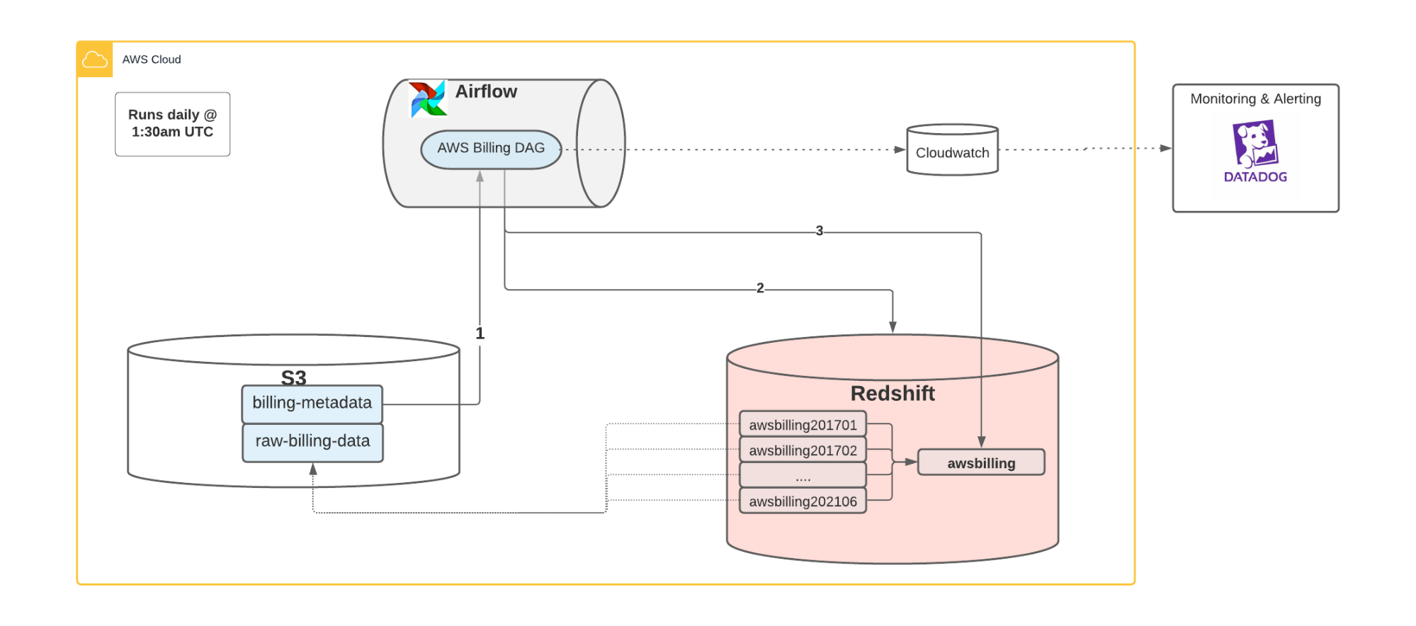
• For every month, we build an external table using Redshift Spectrum that gives us a view into the AWS cost data that exists in S3
• We build a view on top of the external tables to consolidate them into a single place
• We have Logging, Metrics, Alerting, and more using Cloudwatch and Datadog
  

Now that our data was in a common BI storage, we could start to build off of it for our analytics. There were a few things we needed to do first to help us make the most out of our data. 

As we touched on before, the accounting dataset is massive and consists of billions of rows, many of which come from the EC2 instances that host a large part of our platform. Querying this dataset is cumbersome and could be quickly improved by pre-aggregating the data on a daily basis. Instead of always having to query the base accounting dataset with billions of rows and aggregate it every time, querying the aggregated dataset provides the same data but in a fraction of the time. This pre-aggregated dataset became the first of what we call our cost components.

The next thing we wanted to do is start building more cost components to provide us that holistic view we had been trying to achieve. Going back to the SQS example, to build the SQS cost component we pull data from the awsbilling view and the accounting_aggregated component. We also pull in some customer info from another view in Redshift vw_org. We join the three datasets using the CustomerID and filter the awsbilling table for cost information on SQS only.

We have over a dozen of these components with varying levels of complexity all built up and joining between the two main datasets of awsbilling and the accounting_aggregated data while providing filtering or enrichment to the data specific to each component.

Having all of these components was great, and was a huge step up closer to answering our question of “How much does X customer cost us?”. The last thing we needed was to bring all of these components back together into a report view where we can then filter at the customer level instead of at the cost component level.

The data was all in Redshift, and we had separate cost components built for each of our core services. Now, we wanted to expose this data for our business and analytics use cases. Our BI and Analytics tool of choice was Looker. Inside of Looker we have the ability to dive into each cost component as necessary, but also build reports that can answer our initial question: what is our COGS?

One of the most important reports we have is the consolidated view of our AWS Cost. It joins all of the cost components with the accounting data, and breaks it down in multiple ways for easy analysis, allowing for filtering and a quick view into the underlying data.

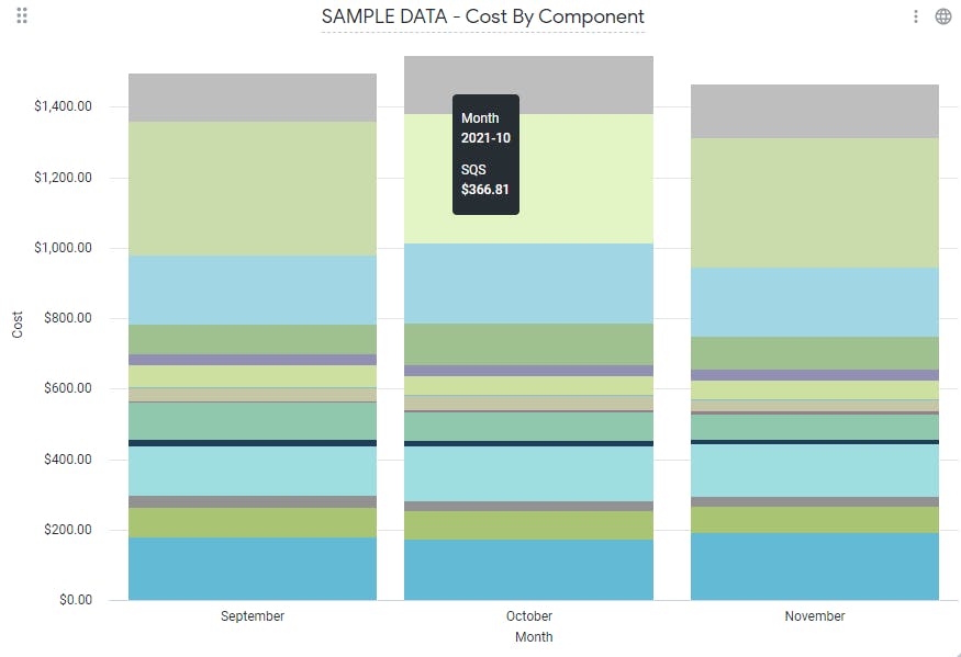
This is where having that common dataset for all of our accounting data and cost components really comes into play.

Having these reports available has been critical to making business decisions and has helped highlight that one of our core components was costing more and more each month as its usage was growing more widespread. This allowed us to take action by forming a squad specifically dedicated to reducing resource consumption and optimizing this component, ultimately cutting its cost down by five times. 

As our platform grows and expands, we can easily build onto this system, adding more components and different breakdowns to the data depending on our needs at the time. Having this data readily available is critically important to making good decisions now, and guiding our decisions as our business grows.