How we cut AWS costs by 80% while usage increased 20%
How do you replace a tire while driving on the highway? This is what it felt like to re-architect the engine behind one of our most heavily used and relied upon products, the mParticle Audience Manager. Here's how we optimized this critical piece of our architecture and positioned it to play a key role in the next phase of our growth, all while customer adoption and usage steadily increased.

The mParticle Audience Manager is one of our core product offerings, allowing our clients to build powerful audience segments to engage their customers with historical context and distribute audience segments for real-time hyper-personalization. The infrastructure that powers the product processes ~200 billion events per month and calculates ~10K audiences in real time.
As the data volume and the number of audiences created in the platform increased over time, the infrastructure cost also increased significantly. In the second half of 2021, we re-architected the audience calculation engine, cut server cost by 80% while the data volume increased by 20%.
The audience system and its code base is one of the most complex systems in our platform, processing large amounts of data in real time. Re-architecting major pieces of it felt like replacing a tire while driving on a highway. Therefore we paid great attention to designing a bulletproof process to roll out the changes.
The chart below shows one of the amazing results we achieved, i.e., cutting the audience calculation latency by almost 20 times which directly resulted in cost savings as we’ll explain later.

Architecture overview
The audience system is responsible for calculating the memberships of all audiences defined in the mParticle platform in near real time. For example, if an audience is defined as “users who have made at least 1 purchase in the last 30 days in the iOS app”, then whenever mParticle receives an event from a user from the iOS app, the audience system needs to count the number of purchase events in the last 30 days and to qualify/disqualify the user. The calculation needs to happen in near real time to enable instant personalization.
As shown in the architecture diagram below, the audience service reads from a message queue where a message contains one or multiple events for a single user (we host our own Pulsar infrastructure), and performs the following actions in sequence:
- Reads the event history and user profile data for the user from Scylla
- Calculates all audiences, whose definitions are read from the cache store
- Stores the event, updates profile data, and stores the audience membership results back to Scylla
- Sends the audience membership results to an output message queue
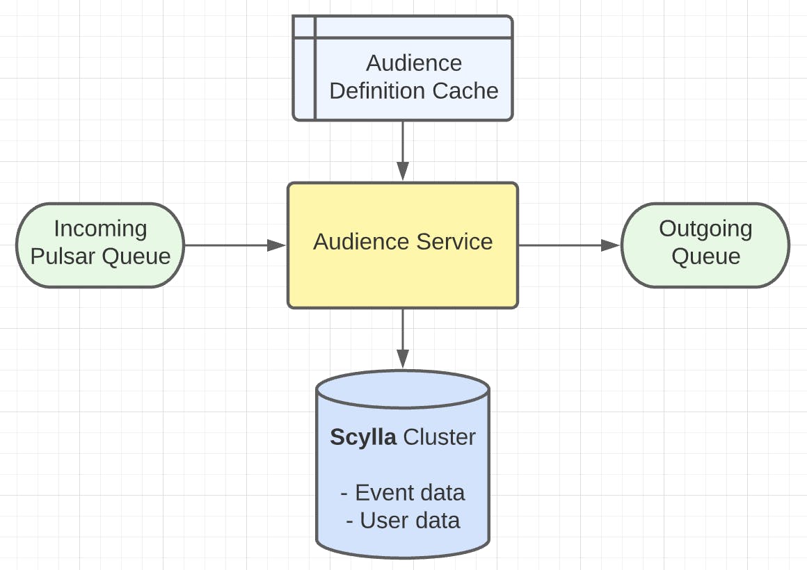
The audience service runs in an AWS ECS cluster and auto-scales to keep up with the incoming messages in real time (~200 billion events per month). Depending on the incoming data rate, there are between 100 and a few thousand docker containers running at any given time.
Why did we need to re-architect?
Re-architecting a system is not always the right plan. In this case, we decided that we needed to re-architect because of issues we were seeing with current and future performance and costs.
Our audience product was first released in 2014 and the core architecture has stayed the same since. As the data volume processed by the system went up dramatically, some of our “good enough” algorithm designs in the calculation engine were not good enough anymore.
Additionally, the processing latency increased as the number of audiences created in the mParticle platform also increased dramatically over the same time period. This was only the beginning - for our next phase of growth we anticipate that the audience engine will play a key role. We needed to invest in improving the efficiency of the audience system so that we will be able to handle many more audiences and support more granular personalization use cases.
We also realized we were reaching diminishing returns as we tried to optimize the cost of the audience system. In the last few years, we’ve monitored the COGS of the audience system closely and have implemented various cost optimizations:
- Minimizing cross-AZ (available zone) traffic as AWS charges $0.01/GB for it
- Optimized auto-scale logic to maximize CPU/memory usage per docker container and optimized ECS container placement to maximize the usage of each EC2 instance
- Various caching tricks to minimize duplicate data access in memory
- Kept the dotnet core version up to date to leverage all performance optimizations
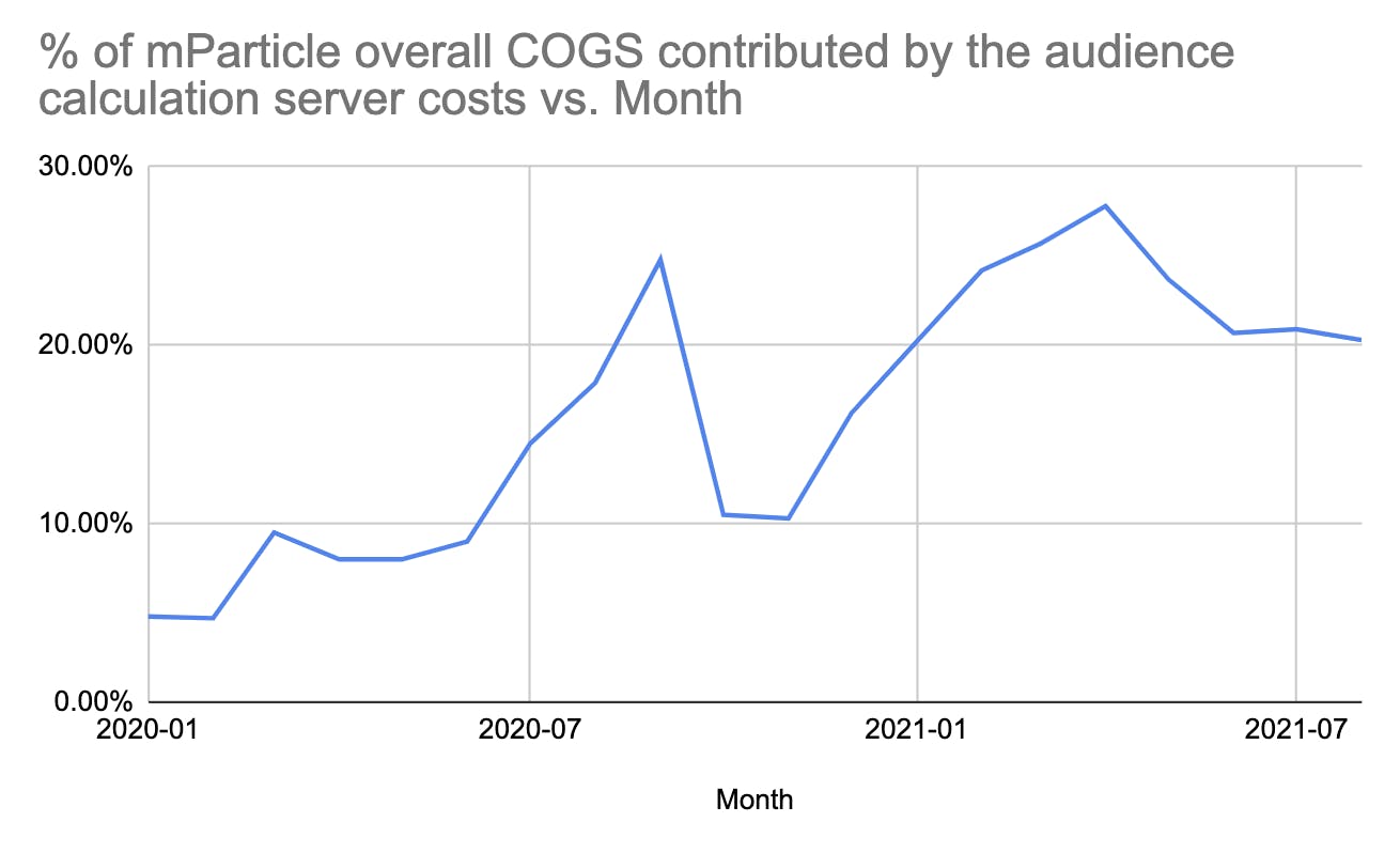
The caching tricks and upgrading dotnet core to 5.0 brought the audience calculation server costs back down to a “normal” level at the end of 2020, as can be seen from the chart below. However, the growth of the data volume combined with the number of audiences persisted in exposing the algorithm inefficiencies in our audience calculation engine, which triggered the re-architecture.
Identify the root cause
Once we had decided we should re-architect the system, our first task was to identify what was at the heart of the performance and cost issues we were battling.
As the audience calculation server costs started going up, we first reviewed all of our previous cost optimizations mentioned above to make sure we didn’t break anything. For example, we confirmed the CPU utilization of each container was still at a decent level. Once we’d ruled out regressions, we investigated our internal metrics in Datadog and concluded that the root cause was the increased calculation latency, which was around 150-300 ms per user per event batch around July 2021. We knew it was the root cause because we saw a strong correlation between the calculation latency and the server costs. Simply put, if each container was spending more time calculating each time we saw a user, then we needed to run more containers at the same time to keep up with the incoming traffic, and therefore higher EC2 cost.
From this root cause analysis, it became clear that we needed to focus on reducing the processing latency.
Once we understood the root cause, we were able to gut check that a re-architecture of the system could get us where we needed to go. To do this, we compared the 150-300 ms per user per event batch processing latency in audience calculation to our Calculated Attribute product, which was performing similar types of calculations in under 10 ms per user per event batch. That gave us confidence that we could significantly reduce the audience product cost if we re-architected the audience engine to be similar to Calculated Attributes.
New audience engine architecture
With a good understanding of the root cause, we were able to determine a new architecture that would better suit our goals for this system, using two main optimization techniques: 1) storing calculation state on a user level and eliminating scanning event history, and 2) micro-batching.
What we needed to optimize
Let’s use an example to help explain where we most needed to optimize with the new architecture. Say we have defined an audience to find users with at least 1 purchase in the last 30 days, and say the current date is 2021/8/26. In the old design, all historical events were stored in an “events” table as follows.
| Timestamp | Event Name | Userid |
|---|---|---|
| 2020/1/16 | Login | 123 |
| 2021/7/15 | Add to cart | 123 |
| 2021/7/12 | Login | 234 |
| 2021/8/1 | View product | 234 |
| 2021/8/2 | Purchase | 234 |
| 2021/8/5 | Purchase | 234 |
When we received new event data on userId 234, we read its event history from the table, processed each of the events, and summed the number of purchases in the last 30 days. In this case there were 2 purchases, and the user qualified for the audience.
If there were N events and M audiences to calculate, the computation complexity for this process was O(NM).
Also, note that the full event history scan was done every time we saw a user. This meant that for any user with a large number of historical events who was seen often, the processing latency would deteriorate quickly.
This system architecture was definitely not ideal, and left us lots of room for improvement. In our new design, we leveraged two optimization techniques: 1) storing calculation state on a user level and eliminating scanning event history, and 2) micro-batching.
Storing calculation state on a user level
In our new design, we saw big wins from optimizing by storing pre-computed calculation state on a user level. Each time we see a user with a new event batch, we read the intermediate calculation state from the “user” table and process the new event into the calculation state, from which we can get the audience membership. Say there are M audiences, the computation complexity is O(M).
For example, the two users above would have calculation states as follows. The userId 234 has a count of purchase events by a certain time interval (in this example, daily), and the userId 123 has an “empty” calculation state since no purchase event has been observed yet.
| Timestamp | Event Name |
|---|---|
| 234 | { “Purchase”: { “2021/8/2”: 1, “2021/8/5”: 1 } } |
| 123 | { “Purchase”: { “Purchase”: null } |
A few notes worth mentioning:
- Storing calculation state eliminates the need for scanning the full event history. However, it sacrifices the accuracy of the calculation because the results are stored at a certain time interval. We could avoid any accuracy loss if we were to use time intervals of length 1 milliseconds, but it certainly would mean a much higher data volume in storage. We’ve decided to use a dynamic time interval creation to balance the accuracy and data storage size. That is, any calculation state would start by using time intervals of small duration, and the duration length would be adjusted up or down to maintain the total number of intervals under a certain threshold. In reality, most users have sparse data and would end up keeping the small time interval length which results in high calculation accuracy.
- In reality, users’ calculation states tend to be sparse, e.g., a lot of users just don’t have any purchase event. Instead of storing a lot of empty calculation states like “Purchase”: null, we’ve applied further optimizations to discard all empty calculation states before storing into Scylla and to recreate the state when needed. This enabled us to cut down the storage space consumption in Scylla by 40% for our big customers.
Micro-batching
In our old architecture, since we calculated audience memberships on every event batch we received in real time, “hot” users could easily cause backlogs. Wouldn’t it be nice to be able to process data in micro-batches (i.e., group data received within a small time window from the same user together and process them all at once)?
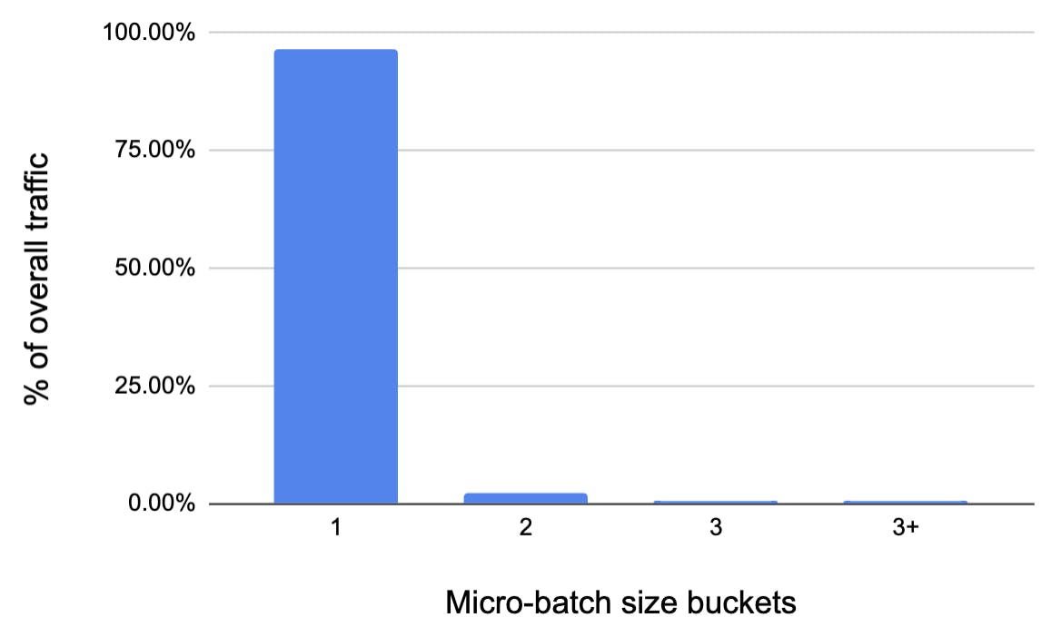
As we migrated our message bus from AWS SQS to Apache Pulsar (another blog post coming soon), we got the benefit of data for a particular user going into the same consumer, which allows us to process micro-batches more easily. To maintain the real-time-ness of the data processing, we currently don’t accumulate much data in memory. The size of micro-batches tend to be 1 most of the time, as shown in the chart below, which helps with “hot” users and cuts down the overall processing load by about 5%.
How we implemented it
Designing a new architecture is one thing, but implementing it is a whole other beast. Here are a few ways that we made sure our implementation would be successful.
Test driven
We’ve written a few thousand unit tests on the audience engine over the years, which gave us a lot of confidence in the correctness of the calculations. However, we did not feel it was enough for a change of this scale. We came up with a list of key use cases in our audience product and spent a few weeks writing a few hundred integration tests that include the audience engine calculations, round trips between the service and the Scylla database, and the dispatching of calculation results. The integration tests caught a few bugs, including some bugs in the old system that we were not aware of.
Local performance testing
Even though the real test of the performance of the new architecture had to be in production at scale, it would speed up the development process and catch any performance issue early on if we had a tool for performance tests locally during the development process. We copied a few thousand audience definitions (no sensitive data was involved since a definition resembles the “more than 1 event in the last 30 days of the eventId 12345 from appId 234” example), and simulated data from some “hot” users to evaluate their audience memberships. This way, we were able to easily compare the calculation latency between the old and the new audience engine code. This meant we didn’t have to instrument additional performance metrics in production nor did we have to debug any performance issues in production, which greatly sped up the development process.
Shadow testing
To further reduce the risks of the re-architecture, we decided to shadow test in production. We ran a small number of canary containers in production. Each container received a small percentage of live traffic, calculated audience memberships using the old engine and the new engine, compared the membership results, and logged any differences for us to investigate. After a few rounds of testing, we were able to resolve all issues.
Controlled rollout with more metrics
To prepare for the rollout of the new architecture, we added a customer level knob to control the % of users going through the new calculation engine, and we added a new dimension, “calculator engine version” (1 = old, 2 = new) in our audience KPI that tracks the number users added to audiences and dropped from audiences at any point in time. This enabled us to roll out the change to one customer at a time and gradually increase the rollout percentage. In the meantime, we monitored the number of adds and drops from each calculator engine version and ensured the ratio matches the rollout percentage, as another validation on the accuracy of the new calculation engine at scale.
For example, the chart below shows the rollout process for one of our customers. The rollout started on 10/4/2021 with 3% of users going to the new version. We gradually increased the % to about 40% on 10/5/2021 and ramped to 100% on 10/7/2021. During the rollout period, we also validated the number of adds and drops by calculator version by audience.

Monitoring
Now that we had spent a few months on the re-architecture, we wanted to build continuous monitoring of the performance to detect any regressions over time. We set up monitoring on the audience calculation latency, which has been holding steady around 5-10 ms.

We also leveraged the automated cost reporting our data services team built in house and monitored the daily cost of the audience calculation servers.
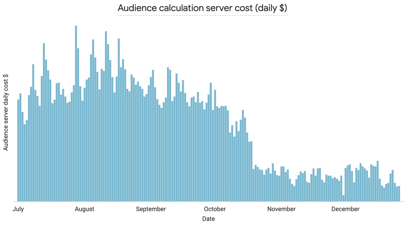
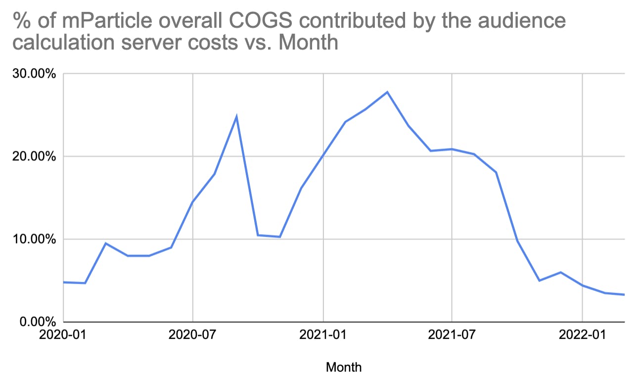
The automated cost reporting also allowed us to see how much the audience calculation server costs contributes to our overall platform COGS. It was exciting to see the big drop in mid October last year!
Future work
Over the years we’ve applied various optimization techniques and architecture changes to our audience system, and this will not be the last. Constantly monitoring system performance, identifying potential bottlenecks, and systematically implementing changes will be a never-ending process. We believe there are a few areas of improvement in the near term:
- Logical reduction of a list of audience definitions to minimize evaluations. An audience definition is represented by criteria combined with logical operators (AND, OR, NOT), and there could be significant room for simplifying the logical definitions within an audience and across audience definitions, especially for some of our big customers where a team of marketers uses our platform and each of them creates their own audiences.
- De-duplicating calculation states across all audience criteria, i.e., if two criteria are like “the number of purchases in the last 30 days” and “the number of purchases in the last 40 days”, we could store one calculation state for the last 30 days and another for the time period 10 days prior, rather than duplicating the data for the last 30 days in two calculation states.
- Minimizing the need to query a user’s full event history as much as possible. For example, indexing event history by event name would allow us to only query for the event names required by an audience definition.
If any of this is interesting to you, please give us your feedback, or come join us to solve similar problems and own part of our infrastructure.


